Anti-Windup PID
Implementing an PID with antiwindup
 Image credit: Author
Note: You can launch this tutorial in live here
![]()
Anti-windup systems
In this notebook we are going to review a simple implementation of anti-windup system for a PID controller based on the classical implementation from (Åstrom,Hägglund, 2005). For better understand the problem of anti-windup, it is useful to implement a regular first order model.
In this case we consider the system:
$$G_1(s) = \frac{1}{\tau s + 1}$$
Notice that when the system is excited with a step response, the classical answer is the solution of the ODE. In the following lines we consider a discretized version of the system, to analyze it’s response.
Notice that the system:
$$G_n(s) = \frac{1}{(\tau s + 1)^n}$$
Is an approximation of a delayed time system of the form
$$G_d(s) = \frac{e^{-sd}}{(\tau s + 1)}$$
For algorithmic purposes we consider $G_{d=4}(s) \approx G_4(n)$
import numpy as np
import matplotlib.pyplot as plt
from sympy import *
# import control as cnt
%matplotlib inline
Let’s the fine the system constants such as sampling time TS and time constant TAU
TS = 0.1 # Sampling time
TAU = 10
class System:

    def __init__(self, K=1):
        self.x = [0]
        self.K = 1
        self.A = 10 # Constant time
        self.T = TS # Sampling time
        self.t = [0]

    def update(self, control):
        """
            Update x_[k+1] as a function of x[k]
        """

        #  Dynamics first order approximation

        x_k = self.x[-1]-\
              self.x[-1]*self.T/self.A + \
              self.K *control*self.T/self.A

        self.x.append(x_k) # State
        self.time_update()

    def time_update(self):
        """ time vector"""
        self.t.append(self.t[-1]+self.T)

    def __call__(self,control):
        """
            Use it like function
        """
        self.update(control)
        return self.x[-1]
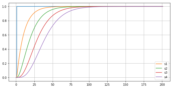
The system evolution can be easily computed in a for loop, in this case we consider $n =4 $
u = np.concatenate([np.zeros(10),np.ones(2000)])

g1,g2,g3,g4 = System(), System(),System(),System()

for ctr in u:
    g4(g3(g2(g1(ctr))))
# Plot of step responses
tu = np.arange(0,(len(u))*TS,TS)
fig, ax = plt.subplots(figsize=(10,5))
plt.plot(tu,u);
ax.plot(g1.t,g1.x,label='s1');
ax.plot(g2.t,g2.x,label='s2');
ax.plot(g3.t,g3.x,label='s3');
ax.plot(g4.t,g4.x,label='s4');
ax.grid(True)
ax.legend();
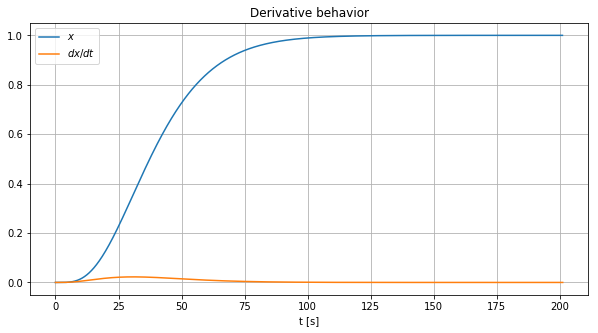
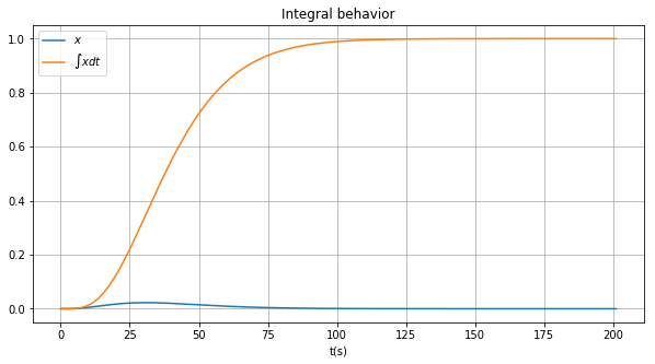
Implementation of derivative and integrals
The following are two simple implementations of a derivative and an integral. The computations are intended for testing purposes.
# %%writefile -a pid.py

class Derivator:
    def __init__(self):
        self.x = [0]
        self.dx = [0]
        self.T = TS
        self.t = [0]

    def diff(self,val):
        """
            Compute (x_k - x_{k-1})/T and updates the memory
        """
        dif = (val - self.x[-1]) / self.T
        self.x.append(val) # memory
        self.dx.append(dif) # memory
        self.time_update()
        return self.dx[-1]

    def time_update(self):
        """ time vector"""
        self.t.append(self.t[-1]+self.T)


    def __call__(self,val):
        """ Call like diff(error) """
        return self.diff(val)
d4 = Derivator()

for sg in g4.x:
    d4(sg)

# Plot and decorations
fig, ax = plt.subplots(figsize=(10,5))
pl=ax.plot(g4.t,g4.x,label='s4');
pl=ax.plot(d4.t,d4.dx,label='d4');
ax.grid(True)
ax.set_title("Derivative behavior")
ax.legend([r"$x$",r"$dx/dt$"])
ax.set_xlabel("t [s]");
# %%writefile -a pid.py

class Integrator:
    def __init__(self):
        self.x = [0]
        self.ix = [0]
        self.T = TS
        self.t = [0]

    def integ(self,val):
        """
            Compute (x_k - x_{k-1})/T and updates the memory
        """
        integral = np.sum(self.T * np.array(self.x))
        self.x.append(val) # memory
        self.ix.append(integral) # memory
        self.time_update()
        return self.ix[-1]

    def time_update(self):
        """ time vector"""
        self.t.append(self.t[-1]+self.T)

    def __call__(self,val):
        """ Call like integ(error) """
        return self.integ(val)
i4 = Integrator()

for sg in d4.dx:
    i4(sg)

fig, ax = plt.subplots(figsize=(10,5))
ax.plot(d4.t,d4.dx,label='dx4');
ax.plot(i4.t,i4.ix,label='i4');
ax.grid(True)
ax.set_title("Integral behavior")
ax.legend([r"$x$",r"$\int{x}dt$"]);
ax.set_xlabel("t(s)");
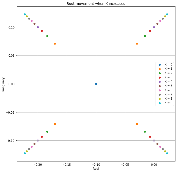
Tunning a PID controller
Here we propose the tunning of the controller via de Ziegler Nichols method. The objective is to find $K_u$ the maximum gain and $T_u$ the oscillation period of the closed loop.

The main point of interest is when $K=4$ since the eigen values become imaginary meaning marginal stability
x = symbols('x')

# Root locus
# sys = cnt.tf([1],coeffs)
# cnt.rlocus(sys);

r_k = []

K =  range(0,10)

# This loop is to find the critical gain K_u

for k in K:
    pol = Poly(expand((10*x+1)**4+k),x)
    coeffs = [float(x) for x in pol.coeffs()]
    r_root = [np.real(v) for v in np.roots(coeffs)]
    i_root = [np.imag(v) for v in np.roots(coeffs)]
    r_k.append((r_root,i_root))

pol = Poly(expand((10*x+1)**4+4),x)
coeffs = [float(x) for x in pol.coeffs()]
roots = np.roots(coeffs)

# Plot and decorations
fig, ax = plt.subplots(figsize=(10,10))
for i,k in zip(r_k,K):
    x,y = i
    ax.scatter(x,y,label=f"K = {k}")
ax.set_title("Root movement when K increases")
ax.set_xlabel("Real")
ax.set_ylabel("Imaginary")
plt.grid(True)
plt.legend();
# System definition
g1,g2,g3,g4 = System(), System(), System(),System()

e = []
r = np.concatenate([np.zeros(10),np.ones(2000)])


for ct in r:
    err = ct - g4.x[-1]
    e.append(err)
    uct = err*4
    g4(g3(g2(g1(uct))))

## Plot and values
tu = np.arange(0,(len(u))*TS,TS)
fig, ax = plt.subplots(figsize=(10,5))
ax.plot(tu,u,label='r');
ax.plot(g4.t,g4.x,label='y');
ax.grid(True,which="both")
ax.legend();
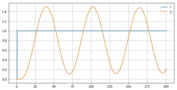
By observation we infer the following values, $K_u$, $T_u$, and we can compute the constants for the PID. Check this link for more info link
# # By observation
K_u = 4 # Critical gain of oscillation
T_u = 70 # By observation

k_p = 0.3*K_u
k_i = 1.2*K_u/T_u
k_d = 3*K_u*T_u/40

print(f"K_p:{k_p}, K_i:{k_i} K_d:{k_d}")
K_p:1.2, K_i:0.06857142857142857 K_d:21.0
Implementing a PID controller
In the following the PID controller will be implemented. The idea is to explain the effects of saturations in the controller and how an antiwindup system may help for that. This full link explains the same idea but in MATLAB link
# %%writefile -a pid.py

class PID:

    def __init__(self, k_p=k_p,k_i=k_i,k_d=k_d):

        # Ziegler Nichols method
        # Check here https://en.wikipedia.org/wiki/Ziegler–Nichols_method
        if k_d == 0:
            self.k_p = 0.45*K_u
            self.k_i = 0.54*K_u/T_u
            self.k_d = k_d
        else:
            self.k_p = k_p
            self.k_i = k_i
            self.k_d = k_d

#         self.k_p = 0.3*K_u
#         self.k_i = 1.2*K_u/T_u
#         self.k_d = 3*K_u*T_u/40

        self.T = TS # Sampling time
        self.t = [0]

        self.u_p = [0]# Proportional term
        self.u_i = [0]# Integral term
        self.u_d = [0] # Derivative term

        self.control = [0]# Control memory

        self.integ = Integrator()
        self.diff = Derivator()


    def apply_control(self,error):

        P = self.k_p * error
        self.u_p.append(P)
        I = self.k_i * self.integ(error)
        self.u_i.append(I)
        D = self.k_d * self.diff(error)
        self.u_d.append(D)

        u_f = self.u_p[-1]+self.u_i[-1]+self.u_d[-1]
        self.time_update()
        self.control.append(u_f)
        return u_f

    def time_update(self):
        """ time vector"""
        self.t.append(self.t[-1]+self.T)

    def __call__(self,error):
        """ Callable """
        return self.apply_control(error)
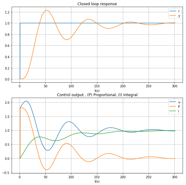
Testing the closed loop system
Let consider the case where a reference is constant and we implement a PI controller. The plots in the figure illustrate the performance of the closed loop system and the effects on the output of the controller and the proportional and integral terms
# System definition
pid = PID(k_d=0)
s1 = System()
s2 = System()
s3 = System()
s4 = System()

e = []
r = np.concatenate([np.zeros(10),np.ones(3000)])

for ct in r:
    err = ct - s4.x[-1]
    e.append(err)
    uct = pid(err)
    s4(s3(s2(s1(uct))))

## Plot and values
tr = np.arange(0,(len(r))*TS,TS)
fig, ax = plt.subplots(2,1,figsize=(10,10))
ax[0].plot(tr,r, label = "r");
ax[0].plot(s4.t,s4.x,label='y');
ax[0].grid(True,which="both")
ax[0].legend();
ax[0].set_xlabel("t(s)");
ax[0].set_title("Closed loop response");

ax[1].plot(pid.t,pid.control, label = "u");
ax[1].plot(pid.t,pid.u_p, label = "P");
ax[1].plot(pid.t,pid.u_i, label = "I");
ax[1].grid(True,which="both");
ax[1].legend();
ax[1].set_xlabel("t(s)");
ax[1].set_title("Control output , (P) Proportional, (I) Integral");
Adding boundaries to the control signal
In the following implementation the output of the controller will be bounded by introducing a saturation before applying to the control

# %%writefile -a pid.py

U_MAX = 10

class PIDlim:

    def __init__(self, k_p=k_p,k_i=k_i,k_d=k_d,u_max=U_MAX):

        # Ziegler Nichols method
        # Check here https://en.wikipedia.org/wiki/Ziegler–Nichols_method
        if k_d == 0:
            self.k_p = 0.45*K_u
            self.k_i = 0.54*K_u/T_u
            self.k_d = k_d
        else:
            self.k_p = k_p
            self.k_i = k_i
            self.k_d = k_d

#         self.k_p = 0.3*K_u
#         self.k_i = 1.2*K_u/T_u
#         self.k_d = 3*K_u*T_u/40

        self.T = TS # Sampling time
        self.t = [0]

        self.u_p = [0]# Proportional term
        self.u_i = [0]# Integral term
        self.u_d = [0] # Derivative term

        self.u_max = u_max
        self.u_min = -u_max

        self.control = [0]# Control memory
        self.control_bnd = [0]

        self.integ = Integrator()
        self.diff = Derivator()


    def apply_control(self,error):

        P = self.k_p * error
        self.u_p.append(P)
        I = self.k_i * self.integ(error)
        self.u_i.append(I)
        D = self.k_d * self.diff(error)
        self.u_d.append(D)

        u_f = self.u_p[-1]+self.u_i[-1]+self.u_d[-1]
        self.control.append(u_f)

        # Bound control
        u_f = max(self.u_min,min(u_f,self.u_max))
        self.control_bnd.append(u_f)

        self.time_update()

        return u_f

    def time_update(self):
        """ time vector"""
        self.t.append(self.t[-1]+self.T)

    def __call__(self,error):
        """ Callable """
        return self.apply_control(error)
pid = PIDlim(k_d=0,u_max=10)
pid1 = PID(k_d=0)

s1,s2,s3,s4 = System(), System(),System(), System()
s5,s6,s7,s8 = System(), System(),System(), System()

e = []
A = 1
r = np.concatenate([A*np.ones(3000),(A+10)*np.ones(3000),A*np.ones(3000)])
tr = np.arange(0,(len(r))*TS,TS)

for ct in r:
    err = ct - s8.x[-1]
    e.append(err)
    uct = pid(err)
    s8(s7(s6(s5(uct)))) # Series system

for ct in r:
    err = ct - s4.x[-1]
    e.append(err)
    uct = pid1(err)
    s4(s3(s2(s1(uct)))) # Series system

## Plot and values

fig, ax = plt.subplots(3,1,figsize=(10,10))
ax[0].plot(tr,r, label = "r");
ax[0].plot(s4.t,s4.x,label='y1');
ax[0].plot(s8.t,s8.x,label='y2');
ax[0].grid(True,which="both")
ax[0].legend([r"$r$",r"$y_{ideal}$",r"$y_{sat}$"]);
ax[0].set_xlabel("t(s)");

ax[1].plot(pid1.t[2:],pid1.control[2:], label = "u");
ax[1].plot(pid.t[1:],pid.control_bnd[1:], label = "ubd");
# # ax[1].plot(pid.t,pid.u_d, label = "D");
ax[1].grid(True,which="both")
ax[1].legend([r"$u_{ideal}$",r"$u_{sat}$"]);
ax[1].set_xlabel("t(s)");

ax[2].plot(pid1.t[2:],pid1.u_i[2:], label = "u");
ax[2].plot(pid.t[2:],pid.u_i[2:], label = "ubd");
ax[2].grid(True,which="both")
ax[2].legend([r"$u_{ideal}$",r"$u_{sat}$"]);
ax[2].set_xlabel("t(s)");
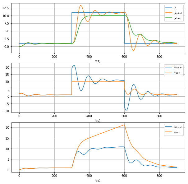
In particular when the change in the reference is very high. The integral term tends to cumulate the error and causing a loss in performance of the output one alternative is to implement a reset of the integrator. The objective will be to reset with a slow time constant via the mechanisms explained in the Amstrom book.

# %%writefile -a pid.py

class PIDantiwindup:

    def __init__(self, k_p=k_p,k_i=k_i,k_d=k_d,u_max=U_MAX):

        # Ziegler Nichols method
        # Check here https://en.wikipedia.org/wiki/Ziegler–Nichols_method
        if k_d == 0:
            self.k_p = 0.45*K_u
            self.k_i = 0.54*K_u/T_u
            self.k_d = k_d
        else:
            self.k_p = k_p
            self.k_i = k_i
            self.k_d = k_d

#         self.k_p = 0.3*K_u
#         self.k_i = 1.2*K_u/T_u
#         self.k_d = 3*K_u*T_u/40

        self.T = TS # Sampling time
        self.t = [0]

        self.u_p = [0]# Proportional term
        self.u_i = [0]# Integral term
        self.u_d = [0] # Derivative term

        self.u_max = u_max
        self.u_min = -u_max

        self.control = [0]# Control memory
        self.control_bnd = [0]

        self.T_t = 1 # Time constant for integration reset

        self.integ = Integrator()
        self.diff = Derivator()


    def apply_control(self,error):

        P = self.k_p * error
        self.u_p.append(P)

        wind_reset = (self.control_bnd[-1] - self.control[-1])/self.T_t

        I = self.integ(self.k_i * error + wind_reset) # Anti windup mechanism

        self.u_i.append(I)
        D = self.k_d * self.diff(error)
        self.u_d.append(D)

        u_f = self.u_p[-1]+self.u_i[-1]+self.u_d[-1]
        self.control.append(u_f)

        # Bound control
        u_f = max(self.u_min,min(u_f,self.u_max))
        self.control_bnd.append(u_f)

        self.time_update()

        return u_f

    def time_update(self):
        """ time vector"""
        self.t.append(self.t[-1]+self.T)

    def __call__(self,error):
        """ Callable """
        return self.apply_control(error)
pid_sat = PIDlim(k_d=0,u_max=10)
pid_windup = PIDantiwindup(k_d=0,u_max=10)

s1,s2,s3,s4 = System(), System(),System(), System()
s5,s6,s7,s8 = System(), System(),System(), System()

e = []
A = 1
r = np.concatenate([A*np.ones(3000),(A+10)*np.ones(3000),A*np.ones(3000)])
tr = np.arange(0,(len(r))*TS,TS)

for ct in r:
    err = ct - s8.x[-1]
    e.append(err)
    uct = pid_sat(err)
    s8(s7(s6(s5(uct)))) # Series system

for ct in r:
    err = ct - s4.x[-1]
    e.append(err)
    uct = pid_windup(err)
    s4(s3(s2(s1(uct)))) # Series system

## Plot and values

fig, ax = plt.subplots(2,1,figsize=(10,10))
ax[0].plot(tr,r, label = "r");
ax[0].plot(s4.t,s4.x,label='y1');
ax[0].plot(s8.t,s8.x,label='y2');
ax[0].grid(True,which="both")
ax[0].legend([r"$r$",r"$y_{no-windup}$",r"$y_{windup}$"]);
ax[0].set_xlabel("t(s)");

ax[1].plot(pid_sat.t[2:],pid_sat.control_bnd[2:], label = "usat");
ax[1].plot(pid_windup.t[1:],pid_windup.control_bnd[1:], label = "uwd");
# # ax[1].plot(pid.t,pid.u_d, label = "D");
ax[1].grid(True,which="both")
ax[1].legend([r"$u_{no-windup}$",r"$u_{windup}$"]);
ax[1].set_xlabel("t(s)");
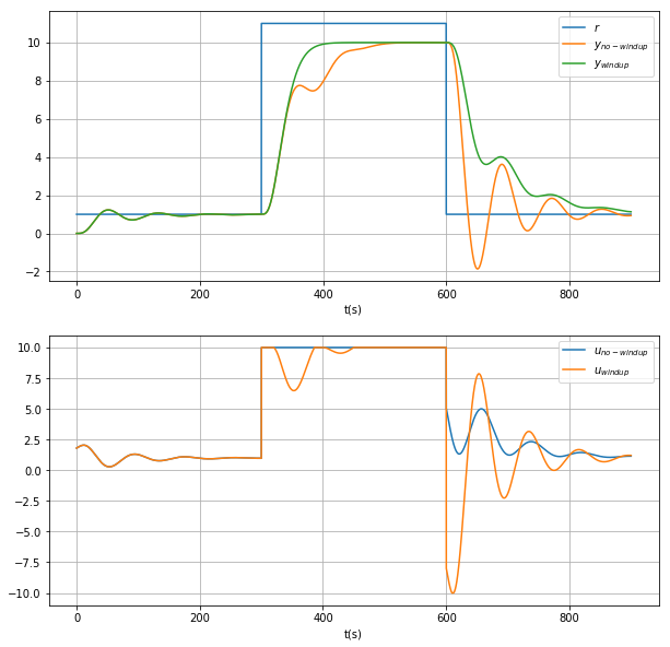
As observed the dynamical response of the system has less overshoot.
Andrés Ladino
Data Scientist
My research interests include distributed control, networked control systems and machine learning.